3D Plot · 三维图#3d-surface#loss-landscape#twin-panel#log-log-axes
Step Law · 3D loss-landscape surface (LR vs. batch-size slices)
Step Law · 3D 损失曲面(LR × BS 双切片)
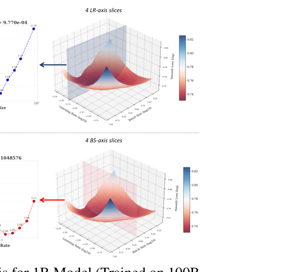
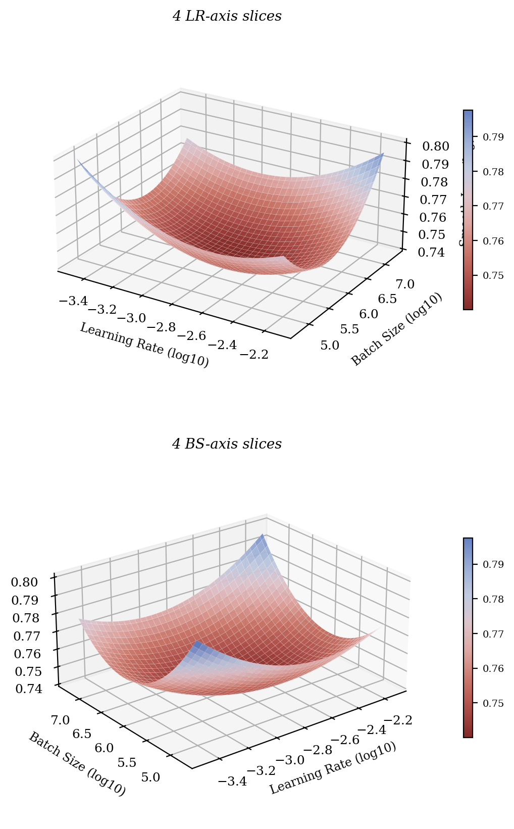
Reproduction of arXiv:2503.04715 Figure 2 (right column). Two stacked 3D surfaces of training loss as a function of (log learning rate, log batch size). The cone-like basin around the empirical optimum is the central message of Step Law. Top panel viewed along the LR-axis slices, bottom along the BS-axis slices. White-meshed surface, red→blue diverging colormap, attached colorbars.
arXiv:2503.04715 Figure 2 右列复现。两幅 3D 损失曲面:以(log Learning Rate, log Batch Size)为底面变量,loss 为高度,呈现一个清晰的反向锥形 basin。上面板沿 LR 轴切片视角,下面板沿 BS 轴切片视角。白色网格曲面 + 红→蓝渐变填色 + 配套色带。
@paper · 来自论文
Predictable Scale: Part I, Step Law — Optimal Hyperparameter Scaling Law in Large Language Model Pre-training
Predictable Scale: Part I, Step Law — 大语言模型预训练的最优超参数缩放律
Houyi Li et al. (StepFun) · arXiv 2025
// original from paper · 论文原图
// reproduced via predictscale_3dloss.py · 脚本复现download png
predictscale_3dloss.py
"""Reproduction of Step Law (Predictable Scale) Figure 2 — 3D loss surface.

Anonymised reproduction of arXiv:2503.04715 Figure 2 right column:
twin 3D surfaces of training loss as a function of (learning rate, batch
size). The inverse-cone shape highlights a single basin around the
empirically observed optimum. Top panel sliced along the LR axis,
bottom panel sliced along the BS axis.

All data is synthesized from a quadratic-in-log-space model anchored at
the published Step-Law optimum (eta* = 1.79 N^-0.713 D^0.307,
B* = 0.58 D^0.571). No checkpoints or training logs are needed.
"""

import numpy as np
import matplotlib.pyplot as plt
from matplotlib.colors import LinearSegmentedColormap
from mpl_toolkits.mplot3d import Axes3D  # noqa: F401  (registers 3D)

plt.rcParams.update({
    "font.family": "serif",
    "font.size": 9,
})

N = 1.0e9
D = 1.0e11
eta_star = 1.79 * (N ** -0.713) * (D ** 0.307)
B_star = 0.58 * (D ** 0.571)

LR = np.logspace(np.log10(eta_star * 0.20), np.log10(eta_star * 4.5), 70)
BS = np.logspace(np.log10(B_star * 0.05), np.log10(B_star * 18), 70)
LRg, BSg = np.meshgrid(LR, BS)

x = np.log10(LRg) - np.log10(eta_star)
y = np.log10(BSg) - np.log10(B_star)
loss = 0.74 + 0.040 * x ** 2 + 0.018 * y ** 2 + 0.012 * x * y

CMAP = LinearSegmentedColormap.from_list(
    "step_law_3d",
    ["#7c1f1c", "#a8443e", "#c66e60", "#dca09b", "#dcc1c9", "#bdc8df", "#94a8d3", "#5e7bc0"],
)

fig = plt.figure(figsize=(8.5, 8.5))

# Top panel — LR-axis sliced surface
ax1 = fig.add_subplot(2, 1, 1, projection="3d")
surf1 = ax1.plot_surface(
    np.log10(LRg), np.log10(BSg), loss,
    cmap=CMAP, edgecolor="white", linewidth=0.06, alpha=0.95, antialiased=True,
)
ax1.set_xlabel("Learning Rate (log10)", fontsize=8.5, labelpad=6)
ax1.set_ylabel("Batch Size (log10)", fontsize=8.5, labelpad=6)
ax1.set_zlabel("Smooth Loss (log)", fontsize=8.5, labelpad=4)
ax1.set_title("4 LR-axis slices", fontsize=10, style="italic", pad=6)
ax1.view_init(elev=24, azim=-58)
ax1.set_box_aspect((1.2, 1.0, 0.55))

cb1 = fig.colorbar(surf1, ax=ax1, shrink=0.55, pad=0.07, aspect=22)
cb1.ax.tick_params(labelsize=7)

# Bottom panel — BS-axis sliced surface (same surface, different camera)
ax2 = fig.add_subplot(2, 1, 2, projection="3d")
surf2 = ax2.plot_surface(
    np.log10(LRg), np.log10(BSg), loss,
    cmap=CMAP, edgecolor="white", linewidth=0.06, alpha=0.95, antialiased=True,
)
ax2.set_xlabel("Learning Rate (log10)", fontsize=8.5, labelpad=6)
ax2.set_ylabel("Batch Size (log10)", fontsize=8.5, labelpad=6)
ax2.set_zlabel("Smooth Loss (log)", fontsize=8.5, labelpad=4)
ax2.set_title("4 BS-axis slices", fontsize=10, style="italic", pad=6)
ax2.view_init(elev=24, azim=-128)
ax2.set_box_aspect((1.2, 1.0, 0.55))

cb2 = fig.colorbar(surf2, ax=ax2, shrink=0.55, pad=0.07, aspect=22)
cb2.ax.tick_params(labelsize=7)

plt.subplots_adjust(hspace=0.18, top=0.96, bottom=0.04, left=0.0, right=0.92)
plt.savefig("predictscale_3dloss_repro.png", dpi=200, bbox_inches="tight")
print("saved predictscale_3dloss_repro.png")