LLM-Evol-Optim · OLS forest plot with confidence intervals
LLM-Evol-Optim · OLS 系数森林图(带 95% 置信区间)
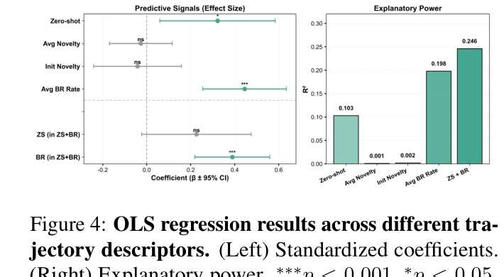
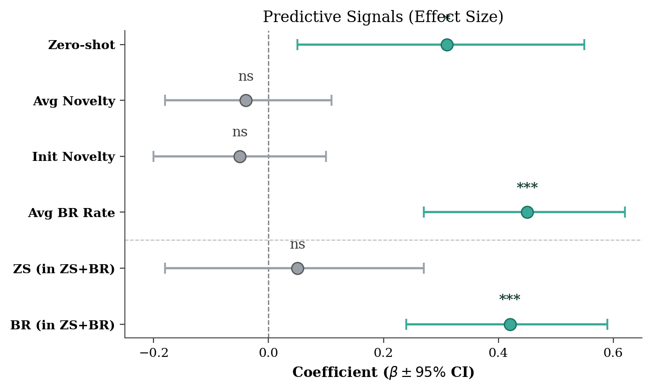
Reproduction of arXiv:2604.19440 Figure 4 (left). Forest plot of standardised OLS regression coefficients (β ± 95% CI) for six trajectory descriptors predicting next-generation breakthrough rate. Significant bars (p < 0.05) are teal with deep-teal markers; non-significant ones (`ns`) are grey. A grey dashed reference line marks β = 0; a horizontal divider separates four single-effect predictors from two interaction terms. Asterisks (`***` / `*` / `ns`) sit above each point.
arXiv:2604.19440 Figure 4 左面板复现。森林图展示六个轨迹描述符对下一代 breakthrough rate 的 OLS 标准化系数(β ± 95% CI)。显著(p < 0.05)的项用青色(深青描边),非显著的(ns)用灰色。虚线竖线标记 β = 0;水平虚线分割上面四个主效应与下面两个交互项。每点上方写显著性星号(*** / * / ns)。
@paper · 来自论文
When Do LLM-Guided Evolutionary Search Trajectories Lead to Breakthroughs?
LLM 引导的进化式搜索何时能带来突破?
LLM-Evol-Optim Authors (Univ. Grenoble Alpes) · arXiv 2026
"""Reproduction of LLM-Evol-Optim Figure 4 (left): forest plot of OLS regression.

Anonymised reproduction of arXiv:2604.19440 Figure 4 (left panel):
A forest plot showing standardised OLS regression coefficients (with 95%
confidence intervals) for six trajectory descriptors predicting next-
generation breakthrough rate. Significant coefficients (p < 0.05) are
drawn with a teal marker; non-significant ones (`ns`) are grey. A grey
dashed reference line marks beta = 0; a horizontal divider separates the
top four single-effect predictors from the bottom two interaction terms.
Asterisks above each point encode p-value bins (*** p<0.001, * p<0.05).

All numbers are inline. No external data is needed.
"""

import numpy as np
import matplotlib.pyplot as plt

plt.rcParams.update({
    "font.family": "serif",
    "font.size": 10,
    "axes.linewidth": 0.7,
})

LABELS = ["Zero-shot", "Avg Novelty", "Init Novelty", "Avg BR Rate",
          "ZS (in ZS+BR)", "BR (in ZS+BR)"]
BETA   = [ 0.31, -0.04, -0.05,  0.45,  0.05,  0.42]
LO     = [ 0.05, -0.18, -0.20,  0.27, -0.18,  0.24]
HI     = [ 0.55,  0.11,  0.10,  0.62,  0.27,  0.59]
SIG    = [True,  False, False, True,  False, True]
STARS  = ["*",   "ns",  "ns",  "***", "ns",  "***"]

y = np.arange(len(LABELS))[::-1]
TEAL = "#3aa996"
GRAY = "#9aa0a8"
EDGE_TEAL = "#1a6e63"

fig, ax = plt.subplots(figsize=(6.6, 4.0))

for i, (b, lo, hi, ok, star) in enumerate(zip(BETA, LO, HI, SIG, STARS)):
    yy = y[i]
    color = TEAL if ok else GRAY
    edge = EDGE_TEAL if ok else "#555"
    ax.errorbar([b], [yy], xerr=[[b - lo], [hi - b]], fmt="none",
                ecolor=color, elinewidth=1.6, capsize=4, capthick=1.3, zorder=3)
    ax.plot([b], [yy], marker="o", markersize=8.5, markerfacecolor=color,
            markeredgecolor=edge, markeredgewidth=0.9, zorder=4, linestyle="none")
    label_color = "#143b34" if ok else "#3a3a3a"
    ax.text(b, yy + 0.30, star, ha="center", va="bottom",
            fontsize=10, color=label_color, fontweight="bold" if ok else "normal")

ax.axvline(0, color="#666", linestyle="--", linewidth=0.9, alpha=0.85)
ax.axhline(y[3] - 0.5, color="#bbb", linestyle="--", linewidth=0.7)

ax.set_yticks(y)
ax.set_yticklabels(LABELS, fontweight="bold", fontsize=9.5)
ax.set_xlabel(r"Coefficient ($\beta \pm 95\%$ CI)", fontsize=10, fontweight="bold")
ax.set_xlim(-0.25, 0.65)
ax.set_xticks([-0.2, 0.0, 0.2, 0.4, 0.6])
ax.set_title("Predictive Signals (Effect Size)", fontsize=11)

for s in ["top", "right"]:
    ax.spines[s].set_visible(False)
ax.spines["left"].set_color("#444")
ax.spines["bottom"].set_color("#444")
ax.tick_params(axis="both", labelsize=9, color="#444")

plt.tight_layout()
plt.savefig("llmoptim_forest_repro.png", dpi=200, bbox_inches="tight")
print("saved llmoptim_forest_repro.png")