Area / Stack · 面积图 / 堆叠图#stacked-area#time-series#category-stack#two-column-legend

AI-Evolution · Stacked area of new architectures by year and domain

AI-Evolution · 各域逐年新架构数堆叠面积图

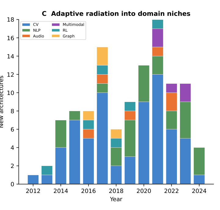
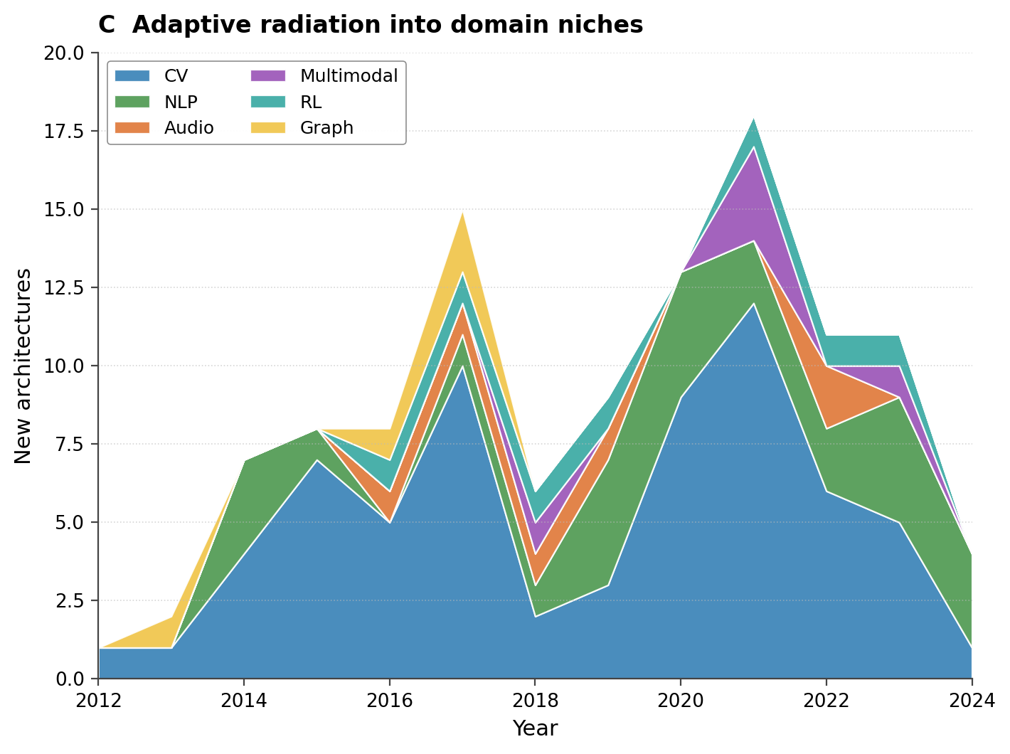
Reproduction of arXiv:2604.10571 Figure 3C as a stacked-area chart (the paper renders the same data as a stacked bar; the area form emphasises the temporal succession of niches). Annual count of new AI architectures from 2012–2024, decomposed into six domain families: CV / NLP / Audio / Multimodal / RL / Graph. Sans-serif, dotted y-grid, two-column upper-left legend.

arXiv:2604.10571 Figure 3C 复现，渲染为堆叠面积图（原文用堆叠柱图，面积形式更强调时序演替）。2012–2024 年每年新增 AI 架构数，按六个领域分层：CV / NLP / Audio / Multimodal / RL / Graph。sans-serif，y 轴虚线网格，左上角双列图例。

@paper · 来自论文

AI Architecture Evolution Mirrors Biological Evolution at Population Scale

AI 架构演化在种群尺度上镜像生物进化

AI Architecture Evolution Authors · arXiv 2026

arXiv:2604.10571 ↗PDF ↗

// original from paper · 论文原图

// reproduced via aievol_diversification.py · 脚本复现download png

aievol_diversification.py

download .py

"""Reproduction of AI-Evolution Figure 3C (stacked architecture origins).

Anonymised reproduction of arXiv:2604.10571 Figure 3C as a *stacked area
chart* (the paper renders the same data as a stacked bar; the area form
emphasises the temporal succession of domain niches).

All counts are inline transcribed from the published figure. No external
data files, APIs, or checkpoints are read.
"""

import numpy as np
import matplotlib.pyplot as plt

plt.rcParams.update({
    "font.family": "sans-serif",
    "font.size": 10,
    "axes.linewidth": 0.8,
})

YEARS = np.array([2012, 2013, 2014, 2015, 2016, 2017, 2018, 2019, 2020,
                  2021, 2022, 2023, 2024])

CV         = np.array([1, 1, 4, 7, 5, 10, 2, 3, 9, 12, 6, 5, 1])
NLP        = np.array([0, 0, 3, 1, 0,  1, 1, 4, 4,  2, 2, 4, 3])
AUDIO      = np.array([0, 0, 0, 0, 1,  1, 1, 1, 0,  0, 2, 0, 0])
MULTIMODAL = np.array([0, 0, 0, 0, 0,  0, 1, 0, 0,  3, 0, 1, 0])
RL         = np.array([0, 0, 0, 0, 1,  1, 1, 1, 0,  1, 1, 1, 0])
GRAPH      = np.array([0, 1, 0, 0, 1,  2, 0, 0, 0,  0, 0, 0, 0])

stacks = np.vstack([CV, NLP, AUDIO, MULTIMODAL, RL, GRAPH])
labels = ["CV", "NLP", "Audio", "Multimodal", "RL", "Graph"]
colors = ["#3a83b8", "#509a52", "#e07a3a", "#9b56b8", "#3aa9a3", "#f0c54a"]

fig, ax = plt.subplots(figsize=(7.2, 5.4))
ax.stackplot(YEARS, stacks, labels=labels, colors=colors,
             alpha=0.92, edgecolor="white", linewidth=0.8)

ax.set_xlim(YEARS.min(), YEARS.max())
ax.set_ylim(0, 20)
ax.set_xticks(np.arange(2012, 2025, 2))
ax.set_xticklabels([str(y) for y in np.arange(2012, 2025, 2)])
ax.set_xlabel("Year", fontsize=11)
ax.set_ylabel("New architectures", fontsize=11)
ax.set_title("C  Adaptive radiation into domain niches",
             fontsize=12, fontweight="bold", loc="left", pad=10)
ax.grid(True, axis="y", linestyle=":", color="#bbb", alpha=0.6, linewidth=0.6)

for s in ["top", "right"]:
    ax.spines[s].set_visible(False)
ax.spines["left"].set_color("#444")
ax.spines["bottom"].set_color("#444")
ax.tick_params(axis="both", labelsize=9.5, color="#444")

leg = ax.legend(loc="upper left", ncol=2, frameon=True, fontsize=9,
                edgecolor="#888", framealpha=0.95)
leg.get_frame().set_linewidth(0.6)

plt.tight_layout()
plt.savefig("aievol_diversification_repro.png", dpi=200, bbox_inches="tight")
print("saved aievol_diversification_repro.png")